Using Histograms to Segment Images

Sometimes it is necessary to seperate an image into segments before running the pieces through optical character recognition. When a document has multiple columns with rows of uneven length it can be a challenge to appropriately attribute one section of the document to one attribute or category.

Below I intend to show a dynamic way to detect sections using my resume. The need for this code came from a past job I worked on that is confidential, but my resume will suffice in showing the concept.

import matplotlib.pyplot as plt
import matplotlib.image as mpimg
import numpy as np
import cv2
import os
from PIL import Image
import warnings
warnings.filterwarnings('ignore')

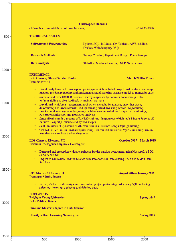
Once you’ve converted your document to an image you can load it into memory using matplotlib.image or python’s opencv. Keep in mind matplotlib.image loads the image as RGB while opencv loads it as BGR.

img = mpimg.imread('C:/Users/cdurrans/Downloads/Data_Scientist_Chris_Durrans_November (1).jpg')
# grayImage = cv2.cvtColor(img, cv2.COLOR_RGB2GRAY) #if you need to transform it to grayscale.
plt.rcParams['figure.figsize'] = [20, 15]
plt.imshow(img)

print("Image minimum:",img.min())
print("Image max:",img.max())
print("Image unique values: ",np.unique(img))

Image minimum: 0
Image max: 255
Image unique values:  [  0   1   2 253 254 255]

We want our image to be binary so we’ll use the following function to make it binary.

(thresh, b_img) = cv2.threshold(img.copy(), 127, 255, cv2.THRESH_BINARY)
print('Unique values: ',np.unique(b_img))
print(b_img)

Unique values:  [  0 255]
[[255 255 255 ... 255 255 255]
 [255 255 255 ... 255 255 255]
 [255 255 255 ... 255 255 255]
 ...
 [255 255 255 ... 255 255 255]
 [255 255 255 ... 255 255 255]
 [255 255 255 ... 255 255 255]]

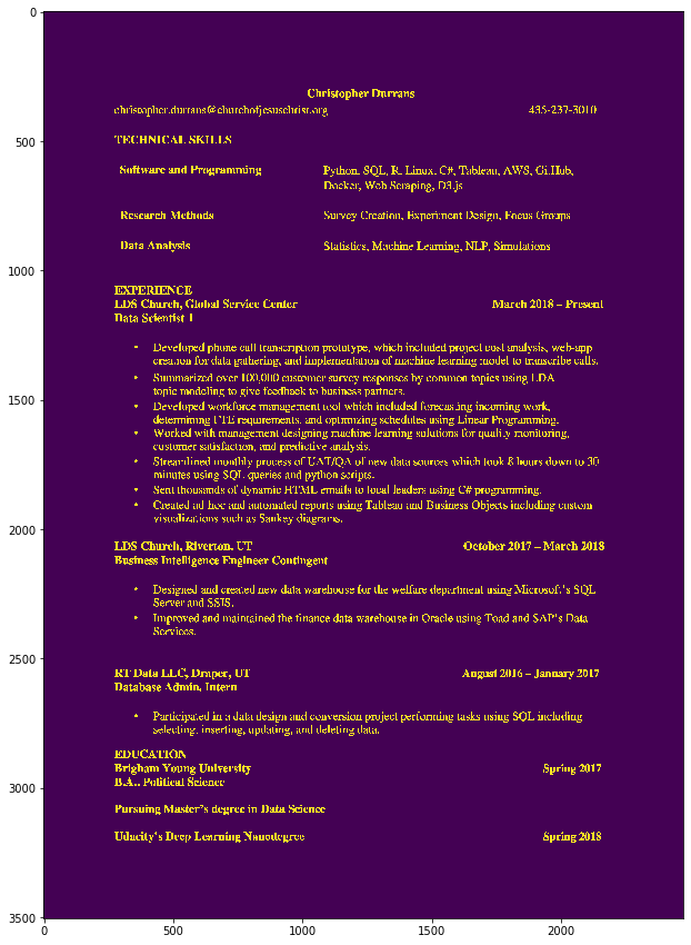
You’ll notice the majority of the image is equal to 255. I prefer to have the reverse and it is better for histogramming images.

b_img[b_img == 0] = 1
b_img[b_img == 255] = 0

plt.imshow(b_img)
plt.show()

When your image is only one channel, all you need to create a histogram of an image is numpy’s sum command! It is really that easy.

#unnecessary but vanity function
def hist(img, axis):
    histogram = np.sum(img, axis=axis)
    return histogram

I’m going to be showing multiple plots side by side so here is a function for that.

def pltMult(pltList,titles=None):
    f, Plts = plt.subplots(1, len(pltList), figsize=(20,10))
    for indx, im in enumerate(Plts):
        if titles != None:
            assert len(pltList) == len(titles)
            im.title.set_text(titles[indx])
        im.plot(pltList[indx])

plt.rcParams['figure.figsize'] = [8, 5]
v_hist_data = hist(b_img,0) # vertical histogram
h_hist_data = hist(b_img,1) # horizontal histogram

pltMult([v_hist_data,h_hist_data],['Vertical Hist.','Horizontal Hist.'])

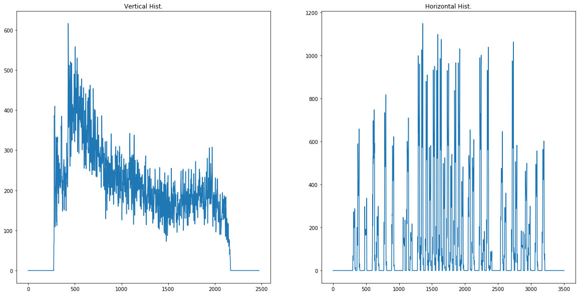
So pay attention to the horizontal histogram. It has many peaks where there is text. I’ve created a function that finds the average index for every valley of zeroes. If we wanted every line we could try using it how it is presently, but we want sections of text. One approach is to calculate the moving average to remove the smallest sections of zeros. I’ll demo below:

def movingAverageHistData(data,rangeToSmooth):
    dataCopy = data.copy()
    for x in range(len(dataCopy)):
        try:
            dataCopy[x] = dataCopy[x-rangeToSmooth:x+rangeToSmooth+1].mean()
        except Exception as ex:
            pass
    return dataCopy

mva12 = movingAverageHistData(h_hist_data,12)
mva5 = movingAverageHistData(h_hist_data,5)
mva20 = movingAverageHistData(h_hist_data,20)

pltMult([mva5,mva12,mva20],['Window 5','Window 12','Window 20'])

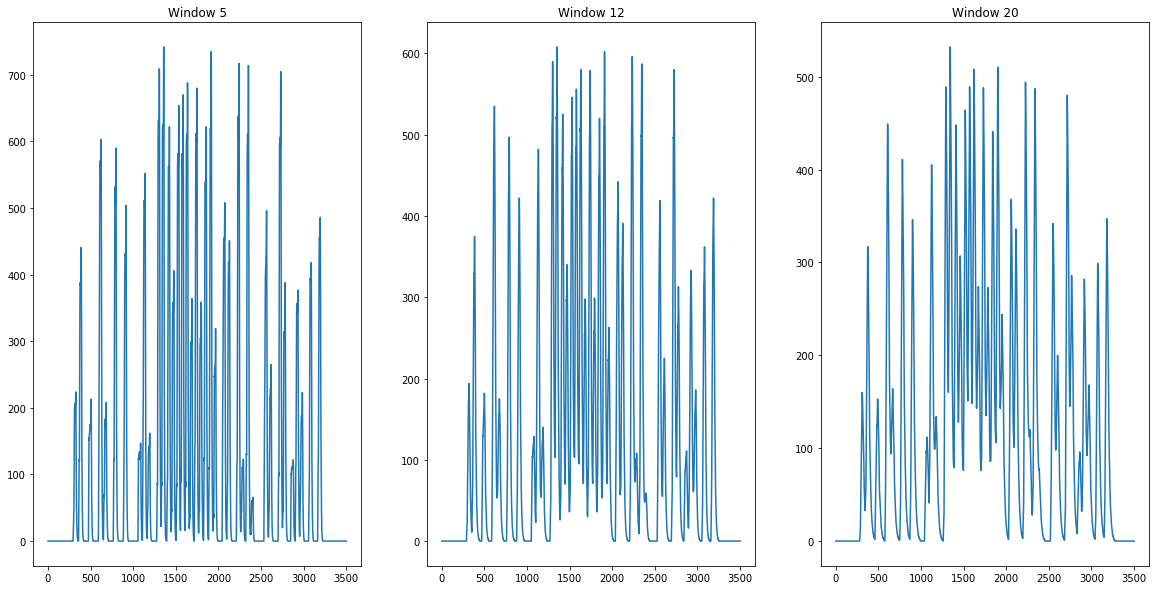
As you can see using different sizes of smoothing windows will reduce the number of segments we’ll seperate.

Below is my implementation for finding the middle of each valley.

def findMiddleOfZeroSections(imgHist):
    lenImage = len(imgHist)
    increaseAmt = 1
    indx = 0
    avgZone = []
    avgZoneCalc = []
    while indx < lenImage:
        if imgHist[indx] == 0:
            avgZoneCalc.append(indx)
            if increaseAmt < 5:
                increaseAmt += 1
        else:
            if avgZoneCalc:
                avgZone.append(int(np.array(avgZoneCalc).mean()))
            avgZoneCalc = []
            increaseAmt = 1
        indx += increaseAmt
    return avgZone

averaged_h_hist = movingAverageHistData(h_hist_data,12)
middleSections = findMiddleOfZeroSections(averaged_h_hist)
print("Indices of valleys: ",middleSections)

Indices of valleys:  [139, 453, 563, 741, 861, 1007, 1248, 2025, 2191, 2480, 2676, 2837, 3039, 3148]

def returnSection(img,sectionIndices,sectionWanted,buffer,verticalOrHorizontal):
    startIndx = sectionIndices[0+sectionWanted]-buffer
    try:
        endIndx = sectionIndices[sectionWanted+1]-buffer
    except IndexError:
        endIndx = len(img)-1
    if verticalOrHorizontal.lower() == 'vertical':
        sectionSeperated = img[:,startIndx:endIndx]
    elif verticalOrHorizontal.lower() == 'horizontal':
        sectionSeperated = img[startIndx:endIndx,:]
    else:
        print("Please enter either vertical or horizontal for verticalOrHorizontal")
        raise ValueError
    return sectionSeperated

plt.rcParams['figure.figsize'] = [12, 8]
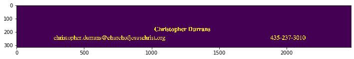
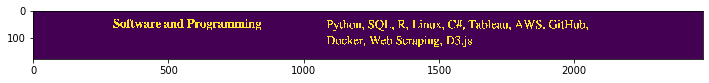
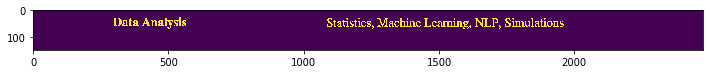
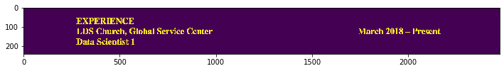
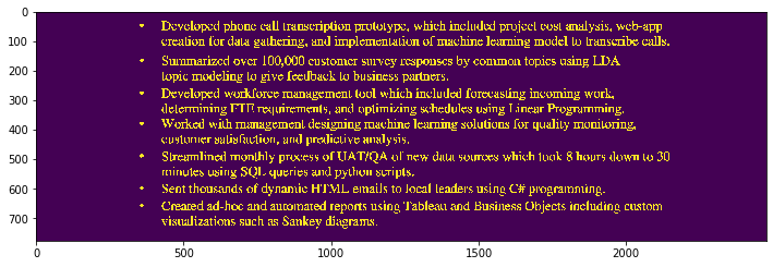
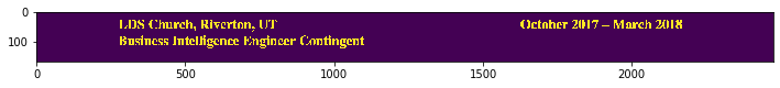
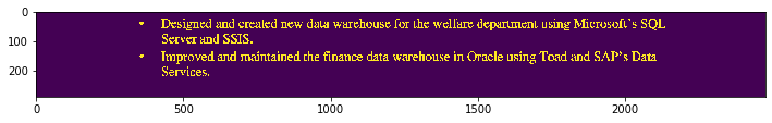
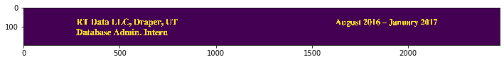
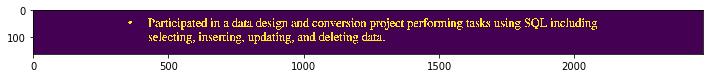
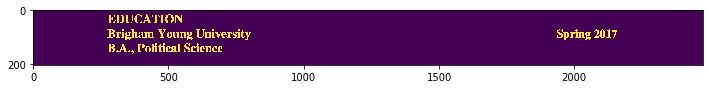
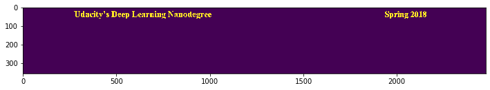
for x in range(len(middleSections)):
    section_x = returnSection(b_img,middleSections,x,0,'horizontal')
    plt.imshow(section_x)
    plt.show()

Conclussion

So as you can see it is a simple technique. Nothing fancy and definitely not perfect, but I hope this inspires you to think of new ways to use simple techniques in your projects. Deep Learning has made amazing strides in tasks such as image segmentation and I’ll do posts on those methods in the future.

#unused function for finding histogram peak every x number of values in hist data.
def getIndicesForTopValuesEveryX(histData, everyX, expectedSections=None):
    """
    Input: given numpy array 
    Process: Find top values for every xth number within an expected number of sections
    output: indices of top values
    """
    if expectedSections == None:
        expectedSections = int(histData.shape[0]/everyX)
    top_nums = []
    for x in range(expectedSections):
        startValue = x*everyX
        results = np.argsort(histData[startValue:(x+1)*everyX])[-1:]
        results += startValue
        top_nums.append(results[0])
    return top_nums