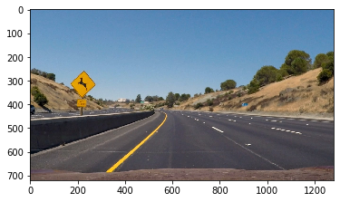
This project is part of Udacity’s self driving car program and the goal is to find lanes on the road and determine car’s position in the lane. For this project I’ll only analyze data coming from one camera centered on the dashboard.

First I’ll import the necessary libraries for exploring these pictures

import matplotlib.pyplot as plt
import matplotlib.image as mpimg
import numpy as np
import cv2
%matplotlib inline

img = mpimg.imread('test_images/test2.jpg')
plt.imshow(img)

I’ll be plotting a lot of images so here is a helper function I created to plot multiple images.

def pltMultImg(images,titles=None):
    f, imagesPlts = plt.subplots(1, len(images), figsize=(20,10))
    for indx, im in enumerate(imagesPlts):
        if titles != None:
            assert len(images) == len(titles)
            im.title.set_text(titles[indx])
        im.imshow(images[indx])

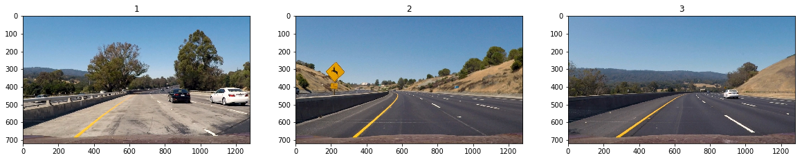
img = mpimg.imread('test_images/test1.jpg')
img2 = mpimg.imread('test_images/test2.jpg')
img3 = mpimg.imread('test_images/test3.jpg')
pltMultImg([img,img2,img3],['1','2','3'])

Step 1 Calibrate Camera When Using a New Camera

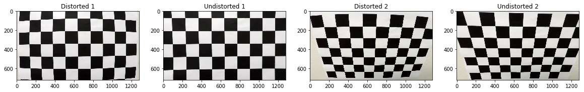
Whenever working with images it is important to understand that every camera causes different kinds and amounts of distortion. Below are shown how objects look distorted when their picture is captured from different angles.

img = mpimg.imread('camera_cal/calibration1.jpg')
img2 = mpimg.imread('camera_cal/calibration2.jpg')
img3 = mpimg.imread('camera_cal/calibration3.jpg')

pltMultImg([img,img2,img3])

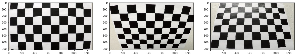
In order to account for distortion we need to take pictures of objects with known dimensions. When we know what the image should look like then we can take many pictures from different angles to later measure the distortion effects and correct for them. Opencv includes some helpful functions such as the cv2.findChessboardCorners, cv2.drawChessboardCorners, and cv2.calibrateCamera to accomplish this task.

# first read in the images, find their corners and object points,
# so that they can be used in the cv2.calibrateCamera function.

import glob
images = glob.glob('camera_cal/calibration*.jpg')

#number of x and y inside corners there are in the chessboards
xNumPts = 9
yNumPts = 6

objpoints = []
imgpoints = []

objp = np.zeros((xNumPts*yNumPts,3),np.float32)
objp[:,:2] = np.mgrid[0:xNumPts,0:yNumPts].T.reshape(-1,2)

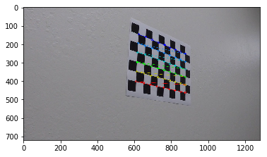
for fname in images:
    img = mpimg.imread(fname)
    gray = cv2.cvtColor(img,cv2.COLOR_BGR2GRAY)
    ret, corners = cv2.findChessboardCorners(gray, (xNumPts,yNumPts),None)
    if ret:
        imgpoints.append(corners)
        objpoints.append(objp)
        img = cv2.drawChessboardCorners(img, (xNumPts,yNumPts), corners, ret)
        plt.imshow(img)

Now that we’ve collected the necessary pieces we can correct for the distortion effects. I’ve included some examples below.

ret, mtx, dist, rvecs, tvecs = cv2.calibrateCamera(objpoints, imgpoints, gray.shape[::-1],None,None)

img = mpimg.imread('camera_cal/calibration1.jpg')
img2 = mpimg.imread('camera_cal/calibration2.jpg')

dst = cv2.undistort(img,mtx,dist,None,mtx)
dst2 = cv2.undistort(img2,mtx,dist,None,mtx)

pltMultImg([img,dst,img2,dst2],["Distorted 1","Undistorted 1","Distorted 2","Undistorted 2"])

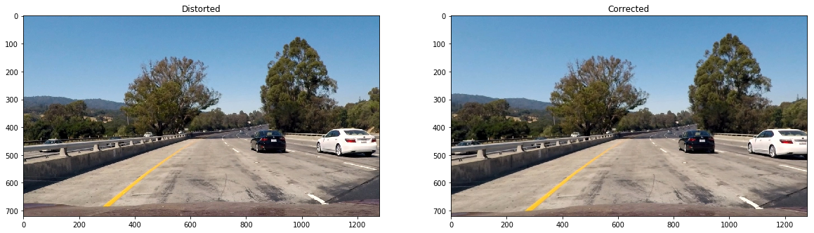
img = mpimg.imread('test_images/test1.jpg')
dst = cv2.undistort(img,mtx,dist,None,mtx)
pltMultImg([img,dst],['Distorted','Corrected'])

Step 2 Feature Extraction and Exploration

Images are rich with color, shapes, and lines which we can use to understand whats in an image. Much of this we take for granted with our eyes and brain, but a computer needs to be told what to look for and how to look for it. Below I’ll walk through some techniques that I’ll be using to detect lines on the road under various road conditions.

# this function uses the absolute value of returned gradients using sobel filters to detect edges
def abs_sobel_thresh(img, orient='x', thresh_min=0, thresh_max=255):
    gray = cv2.cvtColor(img, cv2.COLOR_RGB2GRAY)
    if orient == 'x':
        abs_sobel = np.absolute(cv2.Sobel(gray, cv2.CV_64F, 1, 0))
    if orient == 'y':
        abs_sobel = np.absolute(cv2.Sobel(gray, cv2.CV_64F, 0, 1))
    scaled_sobel = np.uint8(255*abs_sobel/np.max(abs_sobel))
    binary_output = np.zeros_like(scaled_sobel)
    binary_output[(scaled_sobel >= thresh_min) & (scaled_sobel <= thresh_max)] = 1
    return binary_output

# this function finds gradients with certain magnitudes
def mag_threshold(img, sobel_kernel=3, thresh=(0,255)):
    gray = cv2.cvtColor(img, cv2.COLOR_RGB2GRAY)
    sobelx = cv2.Sobel(gray, cv2.CV_64F, 1, 0, ksize=sobel_kernel)
    sobely = cv2.Sobel(gray, cv2.CV_64F, 0, 1, ksize=sobel_kernel)
    magGradient = np.sqrt(sobely**2 + sobelx**2)
    magGradient = (magGradient/ (np.max(magGradient)/255)).astype(np.uint8)
    b_output = np.zeros_like(magGradient)
    b_output[(magGradient >= thresh[0]) & (magGradient <= thresh[1])] = 1
    return b_output

# this function finds gradients with certain directions using arctangent
def dir_threshold(img, sobel_kernel=3, thresh=(0,np.pi/2)):
    gray = cv2.cvtColor(img, cv2.COLOR_RGB2GRAY)
    sobelx = cv2.Sobel(gray, cv2.CV_64F, 1, 0, ksize=sobel_kernel)
    sobely = cv2.Sobel(gray, cv2.CV_64F, 0, 1, ksize=sobel_kernel)
    absgraddir = np.arctan2(np.absolute(sobely), np.absolute(sobelx))
    b_output = np.zeros_like(absgraddir)
    b_output[(absgraddir >= thresh[0]) & (absgraddir <= thresh[1])] = 1
    return b_output
    
# this function uses color channels to find and filter colors
def color_threshold(img, colorTransform=cv2.COLOR_RGB2HLS, channelNum=2, thresh=(0,255)):
    if colorTransform != None:
        tImg = cv2.cvtColor(img, colorTransform)
    else:
        tImg = img
    cChannel = tImg[:,:,channelNum]
    b_output = np.zeros_like(cChannel)
    b_output[(cChannel >= thresh[0]) & (cChannel <= thresh[1])] = 1
    return b_output
    

I created a helper function that combines the output of the filtered images when techniques like those from above are applied.

def combineThresholds(img,binaryResultsList):
    b_combined = np.zeros_like(img[:,:,0])
    for br in binaryResultsList:
        b_combined[(br == 1) | (b_combined == 1)] = 1
    return b_combined

I will show case these functions later. For now I’m going to show color channels.

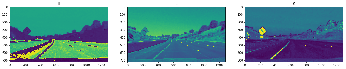
Color Channels

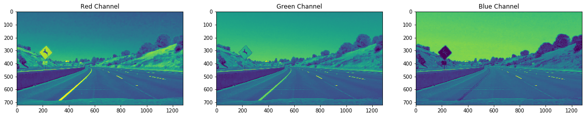
Colors are a powerful way to detect lane lines. Yellow and white lines are easily contrasted against the dark pavement and below I’ll show different colorspaces and we’ll see which will be helpful for finding lanes.

Below I’ve show the red, green, and blue channels that we traditionally think of, but it turns out there are many other color spaces used in computer vision. I’ve included several below and I encourage you to read about them.

#color space filtering
img = mpimg.imread('test_images/test2.jpg')
pltMultImg([img[:,:,0],img[:,:,1],img[:,:,2]],['Red Channel','Green Channel','Blue Channel'])

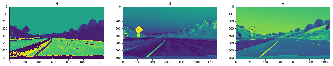
HSV = cv2.cvtColor(img, cv2.COLOR_RGB2HSV)
pltMultImg([HSV[:,:,0],HSV[:,:,1],HSV[:,:,2]],['H','S','V'])

HLS = cv2.cvtColor(img, cv2.COLOR_RGB2HLS)
pltMultImg([HLS[:,:,0],HLS[:,:,1],HLS[:,:,2]],['H','L','S'])

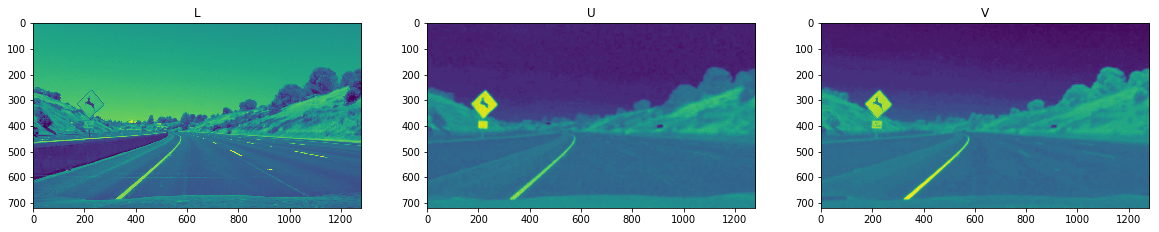
HLS = cv2.cvtColor(img, cv2.COLOR_RGB2LUV)
pltMultImg([HLS[:,:,0],HLS[:,:,1],HLS[:,:,2]],['L','U','V'])

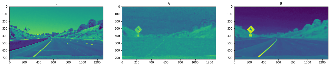
HLS = cv2.cvtColor(img, cv2.COLOR_RGB2LAB)
pltMultImg([HLS[:,:,0],HLS[:,:,1],HLS[:,:,2]],['L','A','B'])

img = mpimg.imread('test_images/test3.jpg')
dst = cv2.undistort(img,mtx,dist,None,mtx)

pltMultImg([dst, 
            color_threshold(dst,cv2.COLOR_RGB2HSV,channelNum=2,thresh=(220,255)), #V Filter
            color_threshold(dst,cv2.COLOR_RGB2HLS,channelNum=2,thresh=(180,255)), #S Filter
            color_threshold(dst,None,channelNum=0,thresh=(220,255)) #Red Filter
           ],['Original','V Filter','S Filter','Red Filter'])

Edge detection

img = mpimg.imread('test_images/test3.jpg')
dst = cv2.undistort(img,mtx,dist,None,mtx)

pltMultImg([abs_sobel_thresh(dst,'x',12,100),
            abs_sobel_thresh(dst,'y',12,100),
            mag_threshold(dst, sobel_kernel=15, thresh=(50,255)),
            dir_threshold(dst,thresh=(np.pi/2.5,(2*np.pi)/2.5))
           ],['Sobel X','Sobel Y','Magnitude','Direction'])

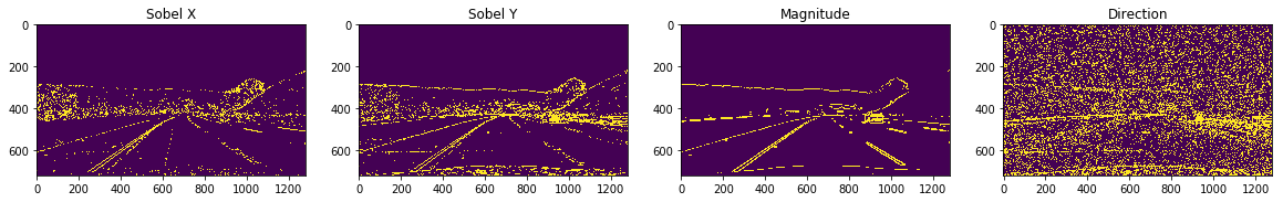
From the above it is easy to see that the color filters and the sobel x and magnitude filters are the most promising. Later in the more difficult situations we’ll see when each of these fail and where they can complement each other to provide a more robust line detector.

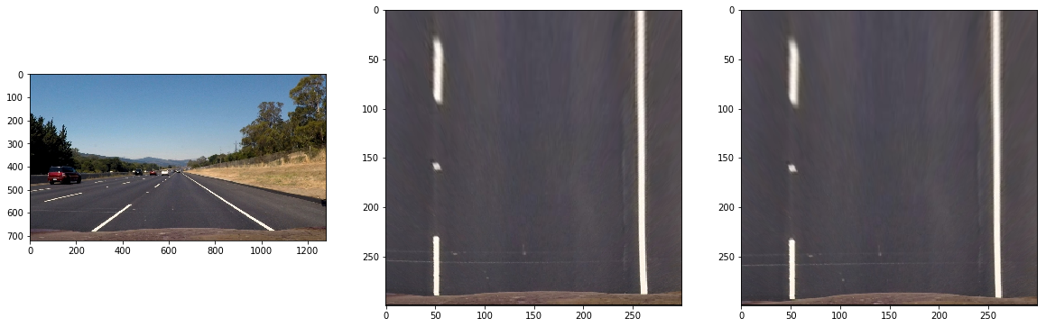
Perspective Transform: Bird’s Eye View

An amazing thing you can do with a little math, is the transformation of an image to make it look like you are looking at an object from another perspective.

Opencv provides the tools for you to select 4 points whether manually or automatically and then transform the perspective so that we can look at the lanes as if we are looking at them from above. With these transformed images we can determine if the lane is curving and by how much.

img = mpimg.imread('test_images/straight_lines2.jpg')
dst = cv2.undistort(img,mtx,dist,None,mtx)

def perspectiveTransformDimensions(img):
    img_size = (img.shape[1],img.shape[0])
    gray = cv2.cvtColor(img, cv2.COLOR_RGB2GRAY)
    ybottom_src = img.shape[0]
    ytop_src = ybottom_src - 250
    xleft_top_src = int(img.shape[1]/3)+100
    xright_top_src = int(img.shape[1]-(img.shape[1]/3))-100
    xleft_bot_src = 0
    xright_bot_src = img.shape[1]
    src = np.float32([[xleft_bot_src, ybottom_src], #bottom left
         [xleft_top_src, ytop_src], #top left
         [xright_top_src, ytop_src], #top right
         [xright_bot_src, ybottom_src]]) #bottom right
    sqSize = 300
    ybottom = 200
    ytop = xleft = ybottom + sqSize
    xright = xleft + sqSize
    
    dst = np.float32(
        [[xleft, ybottom], #bottom left
         [xleft, ytop], #top left
         [xright, ytop], #top right
         [xright, ybottom]] #bottom right
    )
    return src, dst, ybottom,ytop,xleft,xright

def my_perspective_transform(img):
    src, dst, ybottom, ytop, xleft, xright = perspectiveTransformDimensions(img)
    M = cv2.getPerspectiveTransform(src, dst)
    warped = cv2.warpPerspective(img, M, (img.shape[1],img.shape[0]), flags=cv2.INTER_LINEAR)
    return cv2.flip(warped[ybottom:ytop,xleft:xright],0)

pltMultImg([img,my_perspective_transform(img),my_perspective_transform(dst)])

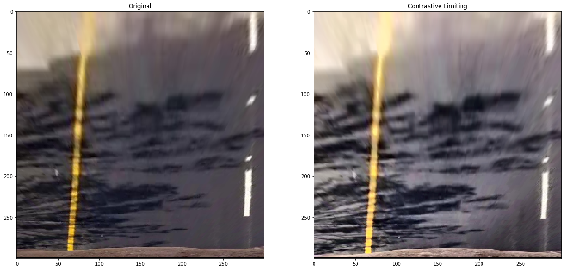
When dealing with shadows sometimes it is useful to use a method called contrastive limiting. Below is a function that applies the technique to colored images.

def contrastiveLimitingColorImage(img):
    lab = cv2.cvtColor(img, cv2.COLOR_RGB2LAB)
    lab_planes = cv2.split(lab)
    clahe = cv2.createCLAHE(clipLimit=2.0, tileGridSize=(8,8))
    lab_planes[0] = clahe.apply(lab_planes[0])
    lab = cv2.merge(lab_planes)
    result = cv2.cvtColor(lab, cv2.COLOR_LAB2RGB)
    return result
#     pltMultImg([img,result])

image = mpimg.imread('treeShadow.jpg')
orig = image
image = cv2.undistort(image,mtx,dist,None,mtx)
image = contrastiveLimitingColorImage(image)
image = my_perspective_transform(image)
pltMultImg([my_perspective_transform(orig),image],['Original','Contrastive Limiting'])

Below is the code for an interactive widget that I used to tune my filters. I spent a fair amount of time filtering and playing with this. One tip: if you want to “turn off” a filter set the low above the high value.

Blog Note: The widget doesn’t work with the blog page. I’ve included the code for your reference, but I’ve removed the output.

from IPython.html import widgets 
from IPython.html.widgets import interact
from IPython.display import display

image = mpimg.imread('treeShadow.jpg')

image = cv2.undistort(image,mtx,dist,None,mtx)
image = my_perspective_transform(image)
image = contrastiveLimitingColorImage(image)
plt.imshow(image)

def combined_binary_mask_interactive(ksize, mag_low, mag_high, dir_low, dir_high, hls_low, hls_high, bright_low, bright_high, red_low, red_high):
    binary_warped = combineThresholds(image,binaryResultsList=[
        mag_threshold(image, sobel_kernel=ksize, thresh=(mag_low,mag_high)),
#         dir_threshold(image, sobel_kernel=ksize, thresh=(dir_low,dir_high)),
        color_threshold(image,cv2.COLOR_RGB2HSV,channelNum=2,thresh=(bright_low,bright_high)),#v1
#         color_threshold(image,cv2.COLOR_RGB2HLS,channelNum=2,thresh=(hls_low,hls_high)),#v1
        color_threshold(image,cv2.COLOR_RGB2LAB,channelNum=2,thresh=(hls_low,hls_high)),#v1
        color_threshold(image,None,channelNum=0,thresh=(red_low,red_high))
    ])
    plt.figure(figsize=(10,10)) 
    plt.imshow(binary_warped,cmap='gray')

interact(combined_binary_mask_interactive, ksize=(1,31,2), mag_low=(0,255), mag_high=(0,255), dir_low=(0, np.pi/2), dir_high=(0, np.pi/2), hls_low=(0,255), hls_high=(0,255), bright_low=(0,255), bright_high=(0,255), red_low=(0,255), red_high=(0,255))

from IPython.html import widgets 
from IPython.html.widgets import interact
from IPython.display import display

#image = mpimg.imread('test_images/test3.jpg')
image = mpimg.imread('bridge1.jpg')

image = cv2.undistort(image,mtx,dist,None,mtx)
image = my_perspective_transform(image)
image = contrastiveLimitingColorImage(image)
plt.imshow(image)

def combined_binary_mask_interactive(ksize, lab_low, lab_high, luv_low, luv_high, bright_low, bright_high, red_low, red_high):
    binary_warped = combineThresholds(image,binaryResultsList=[
        color_threshold(image,cv2.COLOR_RGB2HSV,channelNum=2,thresh=(bright_low,bright_high)),#v1
        color_threshold(image,cv2.COLOR_RGB2LUV,channelNum=0,thresh=(luv_low,luv_high)),#v1
        color_threshold(image,cv2.COLOR_RGB2LAB,channelNum=2,thresh=(lab_low,lab_high)),#v1
        color_threshold(image,None,channelNum=0,thresh=(red_low,red_high))
    ])
    plt.figure(figsize=(10,10)) 
    plt.imshow(binary_warped,cmap='gray')

interact(combined_binary_mask_interactive, ksize=(1,31,2), lab_low=(0,255), lab_high=(0,255), luv_low=(0,255), luv_high=(0,255), bright_low=(0,255), bright_high=(0,255), red_low=(0,255), red_high=(0,255))

Detect lanes from above and identify lanes

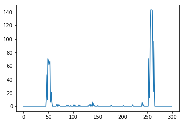
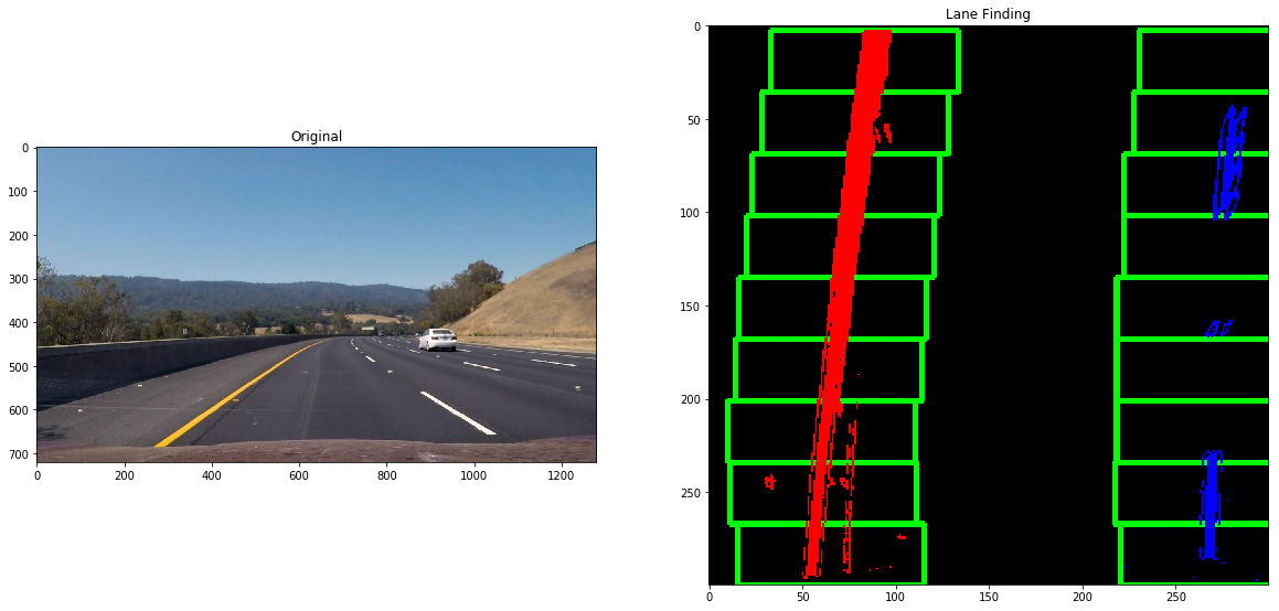
Now we’ll combine the above pieces to detect the lanes and find their curvature. First we’ll correct for distortion, find the lanes, and then plot the histogram of discovered points in the image. Then we’ll run a windowing algorithm that will search segment by segment for where the lane is going from one segment to the next. Then we’ll fit a line to the points and measure its curvature. With the curvature we can determine which direction we are headed and we’ll use that along with points immediately below the camera to determine if we are centered in the lane.

#pipeline for returning lanes from top down view
def warpedBinary(img): #v1
    dst = cv2.undistort(img,mtx,dist,None,mtx)
    warped = my_perspective_transform(dst)
    binary_warped = combineThresholds(warped,binaryResultsList=[
            abs_sobel_thresh(warped,'x',20,100),
            color_threshold(warped,cv2.COLOR_RGB2HSV,channelNum=2,thresh=(220,255)),#v1
            color_threshold(warped,cv2.COLOR_RGB2HLS,channelNum=2,thresh=(180,255)),#v1
            color_threshold(warped,None,channelNum=0,thresh=(220,255))]) #v1
    return binary_warped

def hist(img, half=True):
    if half:
        bottom_half = img[img.shape[0]//2:,:]
    else:
        bottom_half = img
    histogram = np.sum(bottom_half, axis=0)
    return histogram

plt.plot(hist(warpedBinary(img)))

nwindows = 9
margin = 100
minpix = 50

# Load our image
def find_lane_pixels(binary_warped):
    # Take a histogram of the bottom half of the image
    histogram = hist(binary_warped)
    # Create an output image to draw on and visualize the result
    out_img = np.dstack((binary_warped, binary_warped, binary_warped))
    # Find the peak of the left and right halves of the histogram
    # These will be the starting point for the left and right lines
    midpoint = np.int(histogram.shape[0]//2)
    leftx_base = np.argmax(histogram[:midpoint])
    rightx_base = np.argmax(histogram[midpoint:]) + midpoint

    # HYPERPARAMETERS
    # Choose the number of sliding windows
    nwindows = 9
    # Set the width of the windows +/- margin
    margin = 50
    # Set minimum number of pixels found to recenter window
    minpix = 50

    # Set height of windows - based on nwindows above and image shape
    window_height = np.int(binary_warped.shape[0]//nwindows)
    # Identify the x and y positions of all nonzero pixels in the image
    nonzero = binary_warped.nonzero()
    nonzeroy = np.array(nonzero[0])
    nonzerox = np.array(nonzero[1])
    # Current positions to be updated later for each window in nwindows
    leftx_current = leftx_base
    rightx_current = rightx_base

    # Create empty lists to receive left and right lane pixel indices
    left_lane_inds = []
    right_lane_inds = []

    # Step through the windows one by one
    for window in range(nwindows):
        # Identify window boundaries in x and y (and right and left)
        win_y_low = binary_warped.shape[0] - (window+1)*window_height
        win_y_high = binary_warped.shape[0] - window*window_height
        win_xleft_low = leftx_current - margin
        win_xleft_high = leftx_current + margin
        win_xright_low = rightx_current - margin
        win_xright_high = rightx_current + margin
        
        # Draw the windows on the visualization image
        cv2.rectangle(out_img,(win_xleft_low,win_y_low),
        (win_xleft_high,win_y_high),(0,255,0), 2) 
        cv2.rectangle(out_img,(win_xright_low,win_y_low),
        (win_xright_high,win_y_high),(0,255,0), 2) 
        
        # Identify the nonzero pixels in x and y within the window #
        good_left_inds = ((nonzeroy >= win_y_low) & (nonzeroy < win_y_high) & 
        (nonzerox >= win_xleft_low) &  (nonzerox < win_xleft_high)).nonzero()[0]
        good_right_inds = ((nonzeroy >= win_y_low) & (nonzeroy < win_y_high) & 
        (nonzerox >= win_xright_low) &  (nonzerox < win_xright_high)).nonzero()[0]
        
        # Append these indices to the lists
        left_lane_inds.append(good_left_inds)
        right_lane_inds.append(good_right_inds)
        
        # If you found > minpix pixels, recenter next window on their mean position
        if len(good_left_inds) > minpix:
            leftx_current = np.int(np.mean(nonzerox[good_left_inds]))
        if len(good_right_inds) > minpix:        
            rightx_current = np.int(np.mean(nonzerox[good_right_inds]))

    # Concatenate the arrays of indices (previously was a list of lists of pixels)
    try:
        left_lane_inds = np.concatenate(left_lane_inds)
        right_lane_inds = np.concatenate(right_lane_inds)
    except ValueError:
        # Avoids an error if the above is not implemented fully
        pass

    # Extract left and right line pixel positions
    leftx = nonzerox[left_lane_inds]
    lefty = nonzeroy[left_lane_inds] 
    rightx = nonzerox[right_lane_inds]
    righty = nonzeroy[right_lane_inds]

    return leftx, lefty, rightx, righty, out_img

def fit_polynomialDemo(binary_warped):
    # Find our lane pixels first
    leftx, lefty, rightx, righty, out_img = find_lane_pixels(binary_warped)

    # Fit a second order polynomial to each using `np.polyfit`
    left_fit = np.polyfit(lefty, leftx, 2)
    right_fit = np.polyfit(righty, rightx, 2)

    # Generate x and y values for plotting
    ploty = np.linspace(0, binary_warped.shape[0]-1, binary_warped.shape[0] )
    try:
        left_fitx = left_fit[0]*ploty**2 + left_fit[1]*ploty + left_fit[2]
        right_fitx = right_fit[0]*ploty**2 + right_fit[1]*ploty + right_fit[2]
    except TypeError:
        # Avoids an error if `left` and `right_fit` are still none or incorrect
        print('The function failed to fit a line!')
        left_fitx = 1*ploty**2 + 1*ploty
        right_fitx = 1*ploty**2 + 1*ploty

    ## Visualization ##
    # Colors in the left and right lane regions
    out_img[lefty, leftx] = [255, 0, 0]
    out_img[righty, rightx] = [0, 0, 255]
    return out_img

img= mpimg.imread('test_images/test3.jpg')
out_img = fit_polynomialDemo(warpedBinary(img))
pltMultImg([img,out_img],['Original','Lane Finding'])

def fit_poly(img_shape, leftx, lefty, rightx, righty):
     ### TO-DO: Fit a second order polynomial to each with np.polyfit() ###
    left_fit = np.polyfit(lefty, leftx, 2)
    right_fit = np.polyfit(righty, rightx, 2)
    # Generate x and y values for plotting
    ploty = np.linspace(0, img_shape[0]-1, img_shape[0])
    left_fitx = left_fit[0]*ploty**2 + left_fit[1]*ploty + left_fit[2]
    right_fitx = right_fit[0]*ploty**2 + right_fit[1]*ploty + right_fit[2]
    return left_fit, right_fit, left_fitx, right_fitx, ploty

def measure_curvature_real(left_fit,right_fit,y_eval,xm_per_pix=3.7/720, ym_per_pix=30/720):
    '''
    Calculates the curvature of polynomial functions in meters.
    '''
    # Define conversions in x and y from pixels space to meters
    left_curverad = ((1 + (2*left_fit[0]*ym_per_pix*y_eval*ym_per_pix + left_fit[1]*xm_per_pix)**2)**1.5) / np.absolute(2*left_fit[0]*ym_per_pix) 
    right_curverad = ((1 + (2*right_fit[0]*ym_per_pix*y_eval*ym_per_pix + right_fit[1]*xm_per_pix)**2)**1.5) / np.absolute(2*right_fit[0]*ym_per_pix)
    return left_curverad, right_curverad

One of the challenges I came across while working on this is that different filters do well under different situations. In order to explore the many situations I created a debuging video that sped things up significantly.

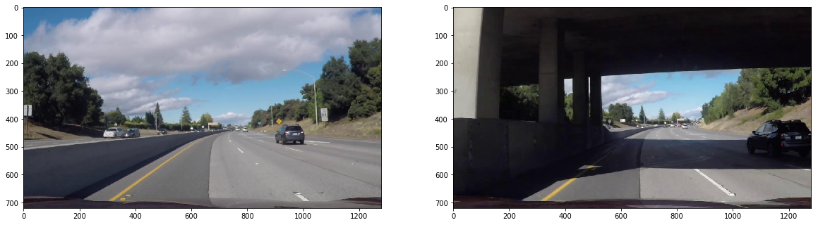
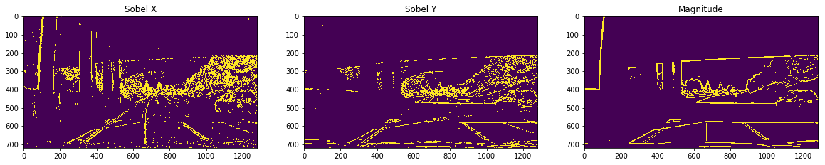
Below is an example of when the gradient methods don’t do as well. When there are dark contrasting lines for example. Many of the color spaces struggle under this dark bridge as well.

half = mpimg.imread('halfRoad.png')
underpass = mpimg.imread('underpass.jpg')
pltMultImg([half, underpass])

pltMultImg([abs_sobel_thresh(underpass,'x',5,100),
            abs_sobel_thresh(underpass,'y',12,100),
            mag_threshold(underpass, sobel_kernel=15, thresh=(50,255))
           ],['Sobel X','Sobel Y','Magnitude'])

In the end I found that the LAB and LUV color spaces do a good job of finding the yellow and white lines under varying lighting conditions.

def warpedBinaryColorOnly(img): #half dark
    dst = cv2.undistort(img,mtx,dist,None,mtx)
    warped = my_perspective_transform(dst)
    img_stack = [
          color_threshold(warped,cv2.COLOR_RGB2LAB,channelNum=2,thresh=(150,255)),#v1,
          color_threshold(warped,cv2.COLOR_RGB2LUV,channelNum=0,thresh=(215,255))#,#v1
    ] # half dark
    binary_warped = combineThresholds(warped,binaryResultsList=img_stack) # half dark
    return binary_warped, img_stack

def inverseTransformDimensions(source_image, destination_image):
    newTarget, dst_, ybottom,ytop,xleft,xright = perspectiveTransformDimensions(destination_image)
    ybottom_src = source_image.shape[0]
    ytop_src = 0
    xleft = 0
    xright = source_image.shape[1]
#     xright = -800
    newSource = np.float32([[xleft, ybottom_src], #bottom left
         [xleft, ytop_src], #top left
         [xright, ytop_src], #top right
         [xright, ybottom_src]]) #bottom right
    return newSource, newTarget

def create_debug_video(img):
    binary_warped, imgStack = warpedBinaryColorOnly(img)
    leftx, lefty, rightx, righty, out_img = find_lane_pixels(binary_warped)
    xm_per_pix = 3.7/700
    ym_per_pix = 30/720
    left_fit, right_fit, left_fitx, right_fitx, ploty = fit_poly(img.shape, leftx, lefty, rightx, righty)
    left_curverad, right_curverad = measure_curvature_real(left_fit,right_fit,img.shape[0],xm_per_pix,ym_per_pix)

    warp_zero = np.zeros_like(binary_warped).astype(np.uint8)
    color_warp = np.dstack((warp_zero, warp_zero, warp_zero))

    # Recast the x and y points into usable format for cv2.fillPoly()
    pts_left = np.array([np.transpose(np.vstack([left_fitx, ploty]))])
    pts_right = np.array([np.flipud(np.transpose(np.vstack([right_fitx, ploty])))])
    pts = np.hstack((pts_left, pts_right))

    justBelowLeft = np.vstack([left_fitx, ploty])[0][0:20]
    justBelowRight = np.vstack([right_fitx, ploty])[0][0:20]

    # Draw the lane onto the warped blank image
    cv2.fillPoly(color_warp, np.int_([pts]), (0,255, 0))
    cv2.polylines(color_warp, np.int_([pts_left]), False, (255, 0, 0), thickness=20)
    cv2.polylines(color_warp, np.int_([pts_right]), False, (0, 0, 255), thickness=20)
    # Warp the blank back to original image space using inverse perspective matrix (Minv)

    newSource, newTarget = inverseTransformDimensions(color_warp, img)
    Minv = cv2.getPerspectiveTransform(newSource,newTarget)
    newwarp = cv2.warpPerspective(color_warp, Minv, (img.shape[1], img.shape[0]), flags=cv2.INTER_LINEAR) 
    result = cv2.addWeighted(img, 1, newwarp, 0.9, 0)
    radCurveTxt = "Radius of Curvature = " + str(int((left_curverad + right_curverad)/2)//10)+" (meters)"
    
    centerPosVal = ((justBelowLeft.mean() + justBelowRight.mean())/2)
    width_midpoint = img.shape[1]//2
    centerPosVal = round(((width_midpoint - centerPosVal) * xm_per_pix)/10,2)
    
    centerPosTxt = "Car is " + str(centerPosVal) + " (meters) off center."
    font = cv2.FONT_HERSHEY_SIMPLEX
    cv2.putText(result,radCurveTxt,(100,100), font, 1, (255, 255, 255), 2, cv2.LINE_AA)
    cv2.putText(result,centerPosTxt,(100,140), font, 1, (255, 255, 255), 2, cv2.LINE_AA)
    vis = result
    
    count = 0
    out_img = np.dstack((imgStack[0], imgStack[0], imgStack[0]))
    output = np.zeros_like(out_img)
    for im in imgStack:
        if count == 0:
            color = 1
        elif count == 1:
            color = 2
        else:
            color = 0
        im = np.dstack((im, im, im))
        im[:,:,color] = im[:,:,color] * 255
        if count == 0:
            output = im            
        else:
            output = np.hstack([output,im])
        count += 1
    
    
    output = cv2.resize(output, (vis.shape[1],vis.shape[0]//2), cv2.INTER_AREA)
    outvis = np.zeros((vis.shape[0]+output.shape[0], vis.shape[1],3))
    outvis[:output.shape[0], :output.shape[1],:] = output
    outvis[output.shape[0]:output.shape[0]+vis.shape[0], :vis.shape[1],:] = vis
    return outvis
    

from moviepy.editor import VideoFileClip
from IPython.display import HTML

white_output = 'project_video_onlyDebug.mp4'
clip1 = VideoFileClip("project_video.mp4")
white_clip = clip1.fl_image(create_debug_video) #NOTE: this function expects color images!!
%time white_clip.write_videofile(white_output, audio=False)
clip1.reader.close()
clip1.audio.reader.close_proc()

[MoviePy] >>>> Building video project_video_onlyDebug.mp4
[MoviePy] Writing video project_video_onlyDebug.mp4


100%|█████████████████████████████████████████████████████████████████████████████▉| 1260/1261 [01:32<00:00, 13.99it/s]


[MoviePy] Done.
[MoviePy] >>>> Video ready: project_video_onlyDebug.mp4 

Wall time: 1min 32s

HTML("""
<video width="960" height="540" controls>
  <source src="{0}">
</video>
""".format('project_video_onlyDebug.mp4'))

Conclusion

The pipeline above does a good job of following the road when the lines are well marked and the road is darker. I would need to tune the values more and potentially use other feature detectors to improve the pipeline for more challenging sections of road. Also in harder videos I’ve tested my current code focuses too far out and looks only straight ahead for lane lines. When the road curves sharply it doesn’t work well at all. In order to address this I could change the perspective transform to shift as the road turns, but I’m hesitant. I think shortening the length in which it looks ahead could help. I’ll leave that for a later date or for the reader to try.